How to Embed a Scrollable Area inside Your Excel Worksheet

If there are a lot of data and information in Excel, it will be cumbersome to view data. Therefore, you can embed a scrollable area in Excel.

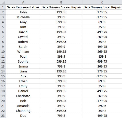
In the image below, you can see the sales volume of many sales representatives. You need to move the worksheet of you want to check other numbers.

Now instead of moving the whole worksheet, you can also embed a scrollable area for this range.

Embed a Scrollable Area in Worksheet

In this part, we will show you the steps to embed such a scrollable area.

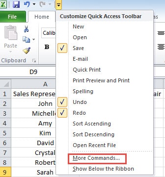
1. Click the small arrow in the quick access toolbar.
2. And then in the drop-down menu, choose the option “More Commands”.
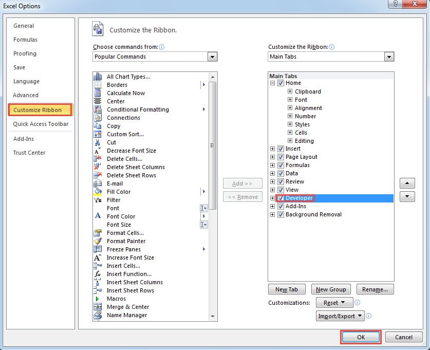
3. In the “Excel Options” window, choose the option “Customize Ribbon” on the left.
4. And the check the tab “Developer” in the “Main Tabs” area.
5. After that, click “OK”. Thus, you have added the tab “Developer” in the ribbon.
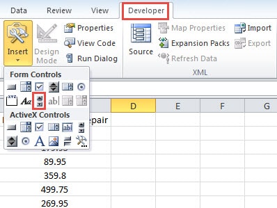
6. Now click this tab in the ribbon.
7. And then click the button “Insert” in the toolbar.
8. In the drop-down list, choose the option “Scroll Bar”.
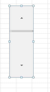
9. And then click in the worksheet. Thus, you have inserted a new scrollbar in the worksheet.
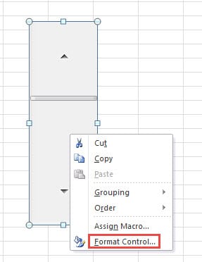
10. Now right click the scroll bar.
11. And then choose the option “Format Control” in the list.
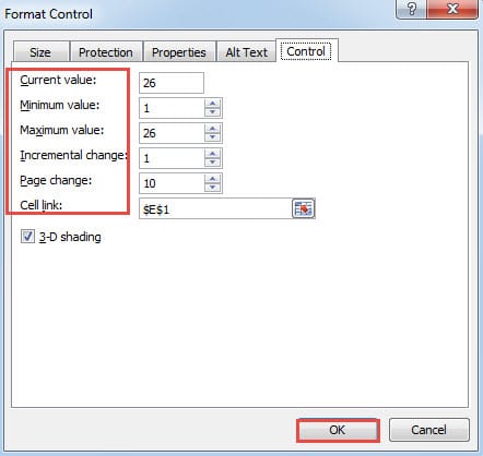
12. In the “Format Control” window, set the corresponding number in those text boxes.

• In the text box of “Current Value”, input the number 1.
• Input the number 1 into the “Minimum value”.
• And then input the maximum value into the corresponding text box. Here you need to input the number according to your actual need. We have 30 rows of numbers, and we want to show 5 rows each time. Thus, the maximum number should be calculated by the formula “=30-5+1”. Here we input “26” in the text box. You can also use this formula to calculate your value.
• Now input the “Incremental change” and the “Page change” according to your need.
• In the “Cell link”, you need to input a cell reference into the text box. You can also use your mouse to select the designated cell.

13. When you finish those settings, click the button “OK”.
14. After that, input the same column header into the area that you need.
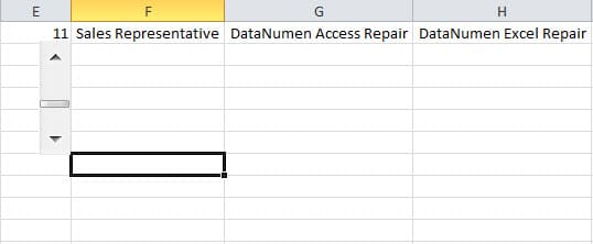
15. And then adjust the size of the scrollbar.
16. Now input this formula into the upper left cell in the scrollable area. In this example, we input the formula into the cell F1.

=OFFSET(A1,$E$1,0)

Here we use the OFFSET function to return the value. A1 is the first cell in the original area. E1 is the link cell that we use for this scrollbar. In this formula, you need to use the absolute for the cell E1.

17. Now use the fill handle to fill other cells in this range. And then you will get the first 5 rows in the range.

Now you can click the arrow in the scroll bar or drag the scrollbar. The numbers in the area will also change according to the current value. Besides, you can also input the current value directly into the link cell. Therefore, you can check the sales volume in a small range.

Save Your Excel with a Powerful Tool

Most of the time, you cannot repair your damaged Excel file by yourself. And incorrect behavior may cause permanent damage to your file. Hence, you can turn to our third party tool for help. This tool can repair xls file corruption in a quick time. And you can get back your files easily.

Author Introduction:

Anna Ma is a data recovery expert in DataNumen, Inc., which is the world leader in data recovery technologies, including repair docx data and outlook repair software products. For more information visit www.datanumen.com