Take your customer satisfaction to the next level. Add your product information along with the price in an Excel workbook and create a shopping cart for your business. All you have to do is share this workbook with your customers and let them select their desired products with a quick preview of billing
Download Now
If you want to start to use the software as soon as possible, then you can:
Otherwise, if you want to DIY, you can read the contents below.
Let’s Prepare the GUI
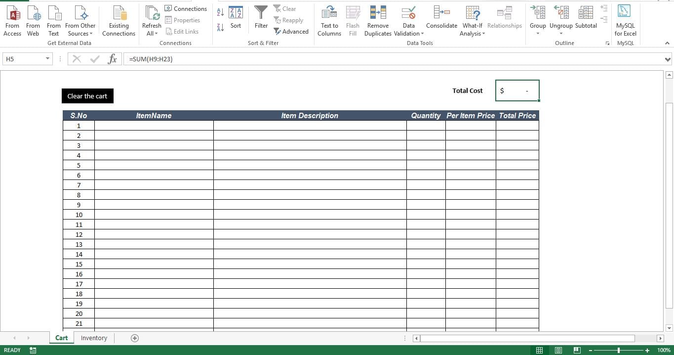
We need 2 sheets. Rename Sheet1 as “Cart” and Sheet2 as “Inventory”. As the name implies, the sheet “Cart” will act as the form where Customers can select an item and add to the cart. Prepare the Cart template by adding necessary headers. For demo purpose, I have added S.No, Item Name, Item Description, Quantity, Per Item Price and Total Price. Also, create 2 more fields to show total items in the cart and the total cost for items in the cart. To make it more professional you can add your company logo and social favicons on this sheet. Insert a shape and name it as “Clear the Cart” button which would be used to empty the cart contents for the user. 
Let’s prepare the database
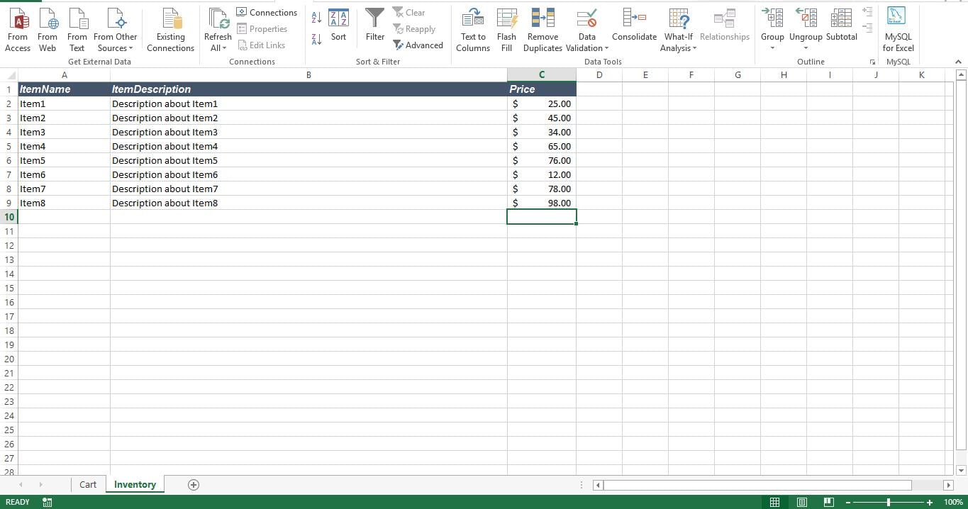
On the Sheet “Inventory” add name, description and per item price of all your products.
Let’s make it functional
We are now going to convert this workbook into a shopping cart by using formulas and data validation. The very first step is to create data validation for the field ItemName on sheet “Cart”. Select the field “ItemName”. Select “Data” tab and then select “Data Validation” inside the group “Data Tools”. Under the tab “Settings”, select the option “List” in the “Allow” box to enable the form to pop out. In the box “Source”, add the address of the range that holds value for our drop down. For this tool, the data sits in the sheet “Inventory”. So the address would be “=Inventory!$A$2:$A$9“. If you are not selecting all cells under the field ItemName, the data validation and the drop down will be applied only to the selected cell.
Now add the following formula to the first cell under the field Item description.
=IF(D9<>"",VLOOKUP(D9,Inventory!A2:B9,2,FALSE),"")
Add the following formula to the first cell under the field Per Item price
=IF(D9<>"",VLOOKUP(D9,Inventory!A2:C9,3,FALSE),"")
Add the following formula to the first cell under the field Total Price
=IF(AND(F9<>"",G9<>""),F9*G9,"")
To display total items in the cart, use this formula
=SUM(F9:F23)
Finally, to display total cost of all items in the cart, use this formula
=SUM(H9:H23)
Add the script to a new module and attach the macro to the button we have created on the sheet “Cart”
How does it work?
As we have data validation on the field “ItemName”, customers can now pick an item from the drop down. Soon as they select an item, using Vlookup, the workbook identifies the corresponding Item description and per item price from the sheet “inventory”. This information is displayed on the sheet “Cart”. When the field “Quantity” is updated, the total price gets populated with correct values. To avoid fields showing “N/A” or “0”, we have added IF statements.
Recover Corrupt Excel files
From time to time, your Excel files with the above shopping cart may get corrupted. In such a case, normally you can consider to use some third-party Excel recovery tool to recover the corrupted files and salvage your data.
Author Introduction:
Nick Vipond is a data recovery expert in DataNumen, Inc., which is the world leader in data recovery technologies, including Word recovery and outlook recovery software products. For more information visit www.datanumen.com
