How to Add Scroll Bars to Your Excel Charts

Chart is a very useful feature in Excel. Therefore, inserting scrollbar into charts can help you better analyze data.

If you need to input a bunch of data into one chart in Excel, you will certainly find that the chart is not easy to look at. And not we have found a new method of inserting scrollbar into a chart in Excel. Thus, you can review the chart more easily.

I. Add Bar Chart and Set Name

1. Select the range that you will use to create a chart.
2. Click the “Insert” tab in the ribbon.
3. Then click the button “Column”.
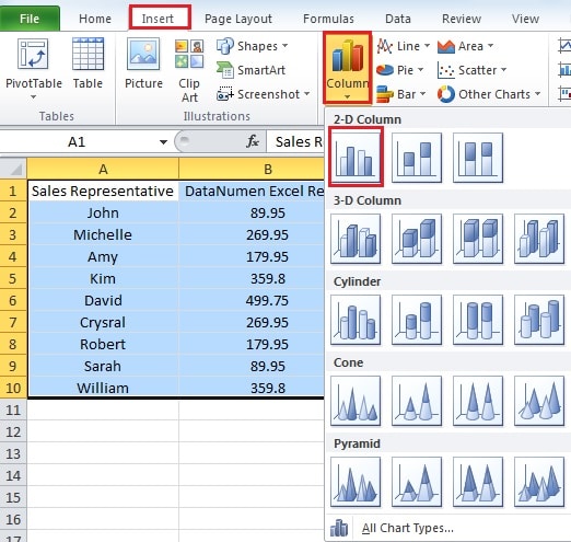
4. And in the drop-down menu, click the chart type. Here we create a bar chart.
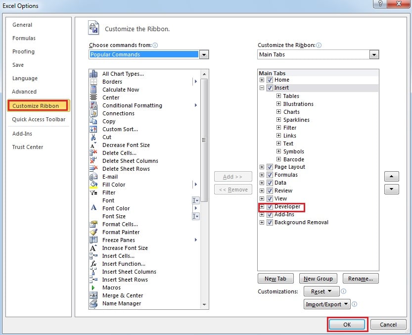
5. Click “File” in the ribbon.
6. And then click “Options”.
7. In the new window, click “Customize Ribbon”.
8. And then in the right part, check the option “Developer”.
9. Then click “OK”. If you have already added this tab, you can skip those steps.
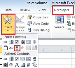
10. Click the “Developer” tab.
11. In the developer tab, click the button “Insert”.
12. And then click “Scroll Bar”.
13. Now you can drag your mouse and draw a scroll bar as your need.
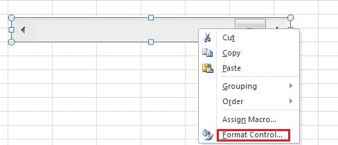
14. After you have created a scrollbar, right click it.
15. In the new menu, choose “Format Control”.
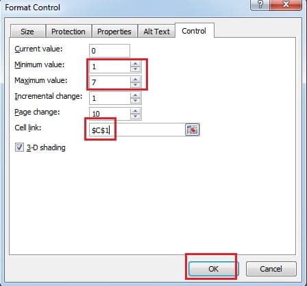
16. In the new window, input the minimum and maximum value.
17. Now you need to input a cell link into the text box. You can set any of a blank as the link cell. And here we set it C1.
18. Then click “OK”.
19. Input the period that you want to show in a blank cell. For example, if you want to show 3 bars in the chart, you can input the number 3. Here we input it into the cell C2.
20. Then click the link cell C1.
21. Click the “Formulas” tab in the ribbon.
22. Then click “Define Name”.
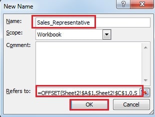
23. Input the name of the first column into the text box. Here we input “Sales_Rperesentative”. If the name includes two words, you should add a “_” between the two words.
24. And then input the formula into the “Refers to” text box:

=OFFSET(Sheet2!$A$1,Sheet2!$C$1,0,Sheet2!$C$2,1)

Sheet2 is the current sheet that you are editing. A1 is the first cell of the range. C1 is the link cell. And C2 is the cell show the period. And you need to change according to your actual situation. The OFFSET function here will return the reference in the text box.

25. Next click “OK”.

26. Now click the “Define Name” once again.

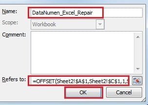
27. In another “New Name” window, input the name into the text box. Here we input “DataNumen_Excel_Repair”.

28. And in the “Refers to” text box. Input this formula:

=OFFSET(Sheet2!$A$1,Sheet2!$C$1,1,Sheet2!$C$2,1)

You should also change it according to your actual situation.

29. And then click “OK”.

II. Set Series in Chart

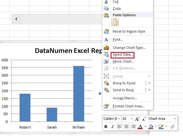
1. Right click the bar chart that you have created before.
2. And in the new menu, then choose “Select Data” option.
3. In the “Select Data Source” window, click “DataNumen Excel Repair”
4. And then click the first “Edit” button on the left.
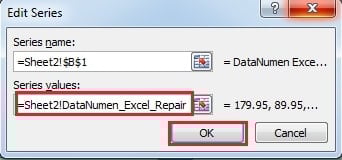
5. Then in the text box of “Series values”, input this into it:

=Sheet2!DataNumen_Excel_Repair

Sheet2 is the sheet that you are now editing. “DataNumen_Excel_Repair” is the name of the second column. Here we add “_” between the words because we have added this in the Name in the previous part. In addition, you need to change the elements according to your worksheet.

6. And then click the button “OK”.

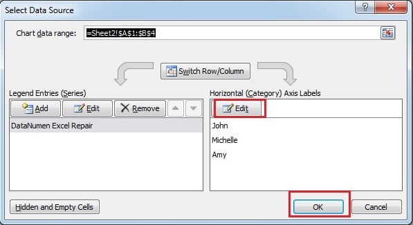
7. Now you will come back to the “Select Data Source” window. Click the second button “Edit” in the “Horizontal (Category) Axis Labels”.

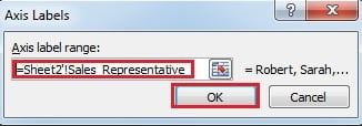
8. Then in the “Axis Labels” window, input this formula into the text box:

=Sheet2′!Sales_Representative

Also you need to change the worksheet and the name.

9. And then click the button “OK”.

10. Then continue clicking “OK” in the “Select Data Source” window.

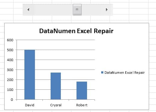
Thus, you have finished all the settings. Now you can click the scroll bar and the category of bars on the chart will also change according to the number. You can also input the numbers directly into the link cell that you have set.

What’s more, the total number of bars will remain 3 as you have set before. And you can also adjust the shape of scroll bar to make it more beautiful. As for the result, you can see the  video below:

You will find that the number on the link cell C1 will also change according to the scroll bar.

Software has Flaws and Excel is Hardly an Exception

Excel is now the most popular software in office. As a result, most of the work needs to use Excel to finish. However, it is still not perfect, like the other software. It will sometimes refuse to work, or you couldn’t open any Excel file. Besides, Excel is also vulnerable to virus and malware. And once the Excel corrupts, the disaster will leave you bewildered. Therefore, you should try to repair it as soon as you can. One of the best Excel recovery tool in the world is our software. It has perfect algorithm and is capable of retrieving almost all the lost data and information in the damaged files.

Author Introduction:

Anna Ma is a data recovery expert in DataNumen, Inc., which is the world leader in data recovery technologies, including word recovery and outlook repair software products. For more information visit www.datanumen.com