4 Quick Methods to Search for Non-Empty Cells in Your Excel Worksheet

Some blank cells in a worksheet are actually not empty. But their existence will make you confused. Therefore, you need to find those non-empty cells in your Excel worksheet.

There are many conditions that a cell will be non-empty while the content in it is invisible. For example, a formula will return null value, the font color in the cell is the same as the fill color, or the invisible values that returned by VBA macros. All those reasons can make the content invisible. But actually those cells are non-empty. And to avoid the problems caused by those cells in your work, you can use the following 4 methods to find those cells that contain invisible contents.

Method 1: Use Ctrl and Arrows Keys

In this method, you need to use the Ctrl and Arrows keys in the keyboard. And below we will demonstrate the thorough step.

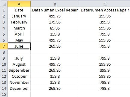
In the image below, there is a blank row in the range.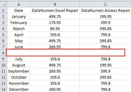

And before deleting the row, you need to make sure that there are no contents in the row. Otherwise some errors will appear and can result in mistakes in other cells.

1. Click the cell A1 in the worksheet.
2. And then press the shortcut keys “Ctrl + ↓” on the keyboard. When you use this shortcut keys combo, the cursor will move to the last non-empty cell in the column.

And in this example, it will move to cell A7. When you press the keys again, the cursor will move to the first non-empty cell in the next range. And in this example, it will move to cell A9. This means that cell A8 is really an empty cell.

3. Now you need to check the second column. Here click the cell B1.
4. And then press the shortcut keys “Ctrl + ↓” again.
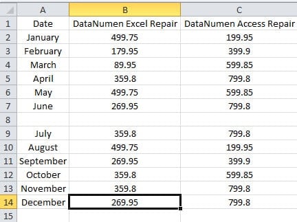
5. After that, see where the cursor position at.

This time, the cursor move to cell B14 directly. This means that cell B8 is a non-empty cell.

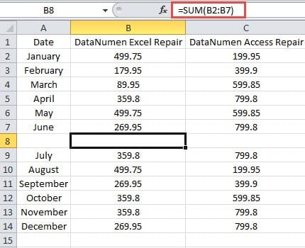
6. Now click the cell B8 and check the value in it. In the formula bar, you can see that there is a formula in the cell.

Here because the font color of the cell is white, so you cannot see it.

7. Now continue using the shortcut keys and check the next column.

When you need to check many cells in a range, clicking those cells one after another and check in the formula bar can be time-consuming. Therefore, you can use this method. Besides, you can also combine other arrow keys with the Ctrl key to check other rows or columns.

Method 2: Use ISBLANK Function

Instead of using shortcut keys, you can also use the ISBLANK function in your worksheet.

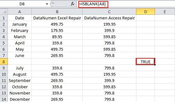
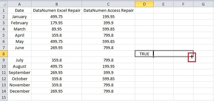
1. Click a blank cell in the worksheet. In this example, we click cell D8.
2. And then input the formula into the cell.

=ISBLANK(A8)

3. Next press the button “Enter” on the keyboard. Thus, you will get a result in this cell.

Here the formula returns a result “TRUE” in the cell.

4. Now click the fill handle of the cell and drag rightward to fill other cells.

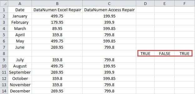
And then you will see all the result for the three cells. You can see that the result in cell E8 is “FALSE”, which means that cell B8 is a non-empty cell.

You can see that using this function is very easy. When you need to check for a whole column or a whole row, you can use this method quickly.

Method 3: Use Conditional Formatting

In this method, you can also use conditional formatting to highlight certain cells. Here you can highlight the empty cells in a range.

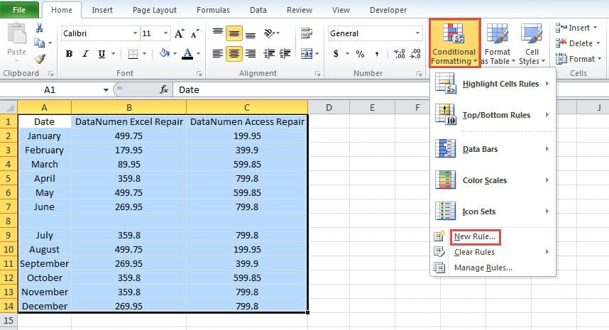
1. Select the target range that contains all the target cells.
2. And then click the button “Conditional Formatting”.
3. After that, in the drop-down menu, choose the option “New Rule”.
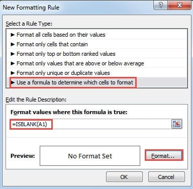
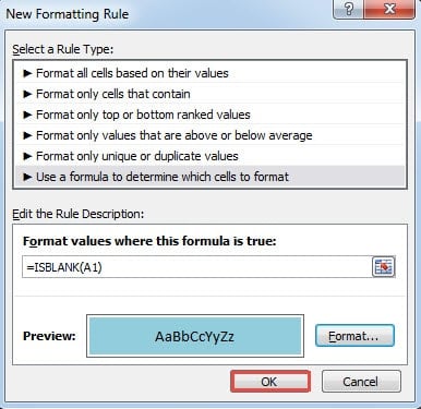
4. In the “New Formatting Rule” window, choose the last option that needs to use formula.
5. Now input the formula into the text box:

=ISBLANK(A1)

Here you will also use the ISBLANK function. Here make sure that the cell is the first cell in the range. On the other hand, if you need to highlight non-empty cells in a range, you can input this formula:

=NOT(ISBLANK(A6))

6. And then click the button “Format”.
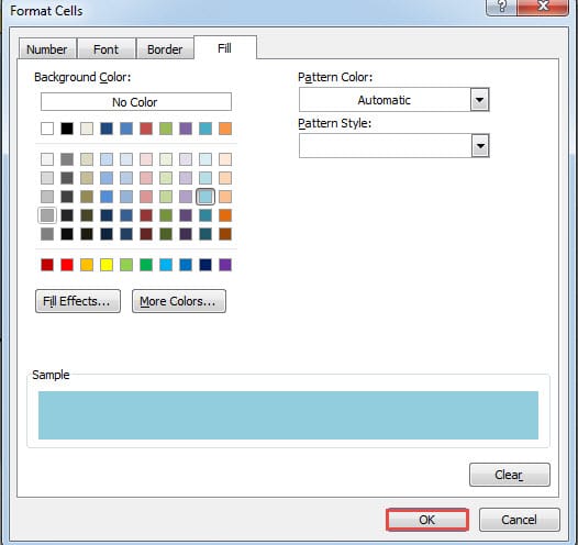
7. In the “Format Cells” window, set a format for the cell.
8. When you have finished the setting, click the button “OK”.
9. Next click “OK” in the “New Formatting Rule” window.

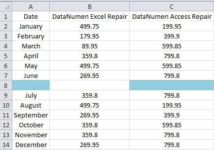
And then you can see that in the range, true empty cells will be highlighted.

Hence you can know that the cell B8 contains a value. Using conditional formatting can also help you judge those cells quickly.

Method 4: Use VBA Macro

This is the last method and you will use the VBA macros.

1. Press the shortcut keys “Alt +F11” on the keyboard to open the VBA editor.
2. And then click the button “Insert” in the toolbar.
3. After that, choose the option “Module” in the sub menu. Thus, you have inserted a new module into the file.
4. Now copy and paste the following codes into the module.

Sub findcell()

    Dim cel As Range

    For Each cel In Range(“A1:C14”)

        If IsEmpty(cel) = True Then

            cel.Interior.Color = vbYellow

        End If

    Next cel

End Sub

Here we will also find the empty cells and format them. If you need to format cells that contain contents, you can also modify the codes according to your need. You may also pay attention that you need to clear all the conditional formatting. Otherwise the format of VBA macro will be covered by the format of conditional formatting. And this will cause trouble to you.

5. Now click the button “Run Sub” in the toolbar or press the button “F5” on the keyboard to run this macro.
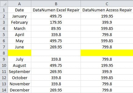
6. After that, come back to the worksheet. And you will see the result like the image below shows.

The formats of real empty cells change. Therefore, cell B8 is a non-empty cell in this range.

A Comparison between the Methods

Here we have listed the advantages and disadvantages of the above four methods.

Comparison	Ctrl and Arrows Keys	ISBLANK Function	Conditional Formatting	VBA Macro
Advantages	You can apply this method quickly when you need to find non-empty cells in a row or a column.	When you need to judge cells in a range, this function is very helpful.	All the result can be listed clearly in the worksheet. And you can choose to format empty cells or non-empty cells according to your need.	With just one click, you can easily get the result. Besides, you can also modify the codes according to your need.
Disadvantages	Compared with other methods, this method will be time-consuming.	If the non-empty cells are separate in different position, it will be inconvenient to use this formula.	The format of conditional formatting will interfere with other cell formats.	If you are not familiar with Excel VBA, the task will be more complicated.

From the above analysis, you will have a comprehensive understanding of the four methods. And you can choose the most suitable method according to your need.

Protect Your Excel Files

The safety of mission-critical Excel files in your storage devices is very essential. Therefore, you need to carefully protect your Excel files. The Excel files have long been victim to malicious virus and malware. Whenever you find Excel corruption in your computer, you need to take the right actions. And you can also use a recovery tool to repair Excel file. In all the methods that can deal with Excel errors, using a tool is the most cost-effective method.

Author Introduction:

Anna Ma is a data recovery expert in DataNumen, Inc., which is the world leader in data recovery technologies, including repair docx data problem and outlook repair software products. For more information visit www.datanumen.com