Sometimes you need to show or hide gridlines to fulfill some tasks. Here we will provide 3 quick methods to show or hide gridlines easily.
In your Excel worksheet, the gridlines can help you distinguish different cells. But on the other hand, sometimes you don’t need the gridlines. Therefore, you need to hide them. Below are the 3 different methods that you can apply.
Method 1: Use Features in Toolbar
There are two different places in the toolbar that you can show or hide gridlines. Here we will introduce one by one.
- Click the tab “Page Layout” in the ribbon.
- And then uncheck the option “View” in the “Sheet Options” of the “Gridlines”. If you need to show the gridline, you need to check the option here.
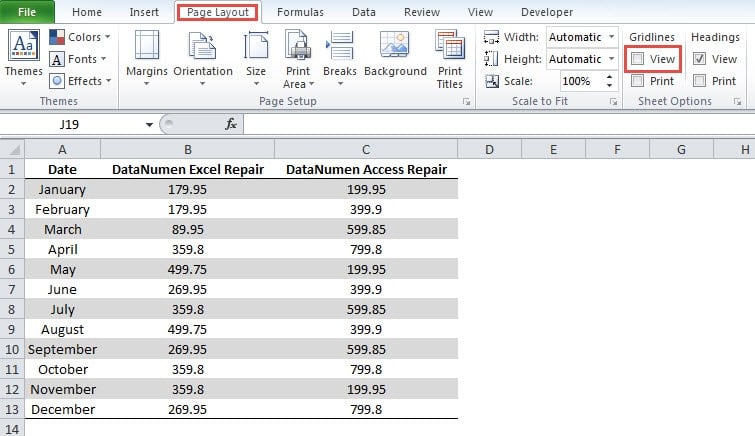
Thus, the gridline will hide or show according to your setting.
Below we present the steps of using another option.
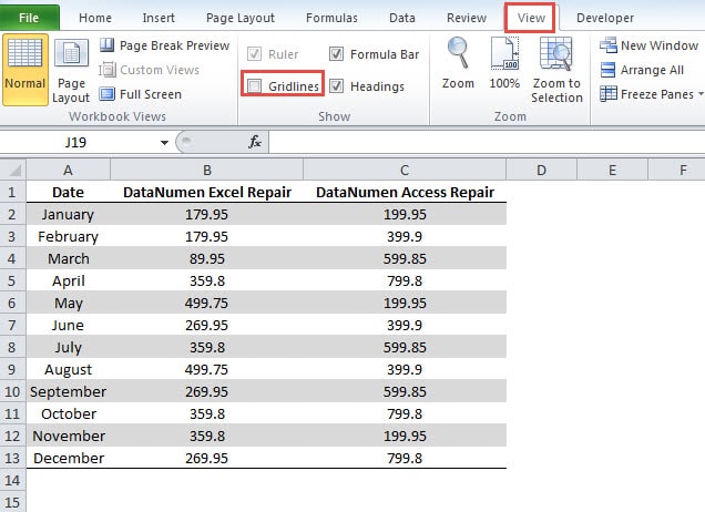
- Click the tab “View” in the ribbon.
- And then uncheck the option “Gridlines” to hide them. Besides, if you need to show gridlines, you need to check the options here.
And the gridline will show or hide according to the setting in the toolbar. These two options have the same effect. You can use either of them according to your habit.
Method 2: Add Buttons in the Quick Access Toolbar
Instead of using the previous method, you can also add buttons in the quick access toolbar.
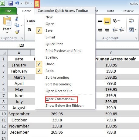
- Click the small arrow in the quick access toolbar.
- And then select the option “More Commands”.
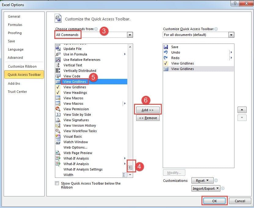
- In the “Excel Options” window, choose the option “All Commands” for the “Choose commands from”.
- And then drag the scrollbar until you see the options about gridlines”.
- There are two different options about gridlines. Here we add both into the toolbar. First click one of the options.
- And then click the button “Add”.
- Next repeat the steps and add another button.
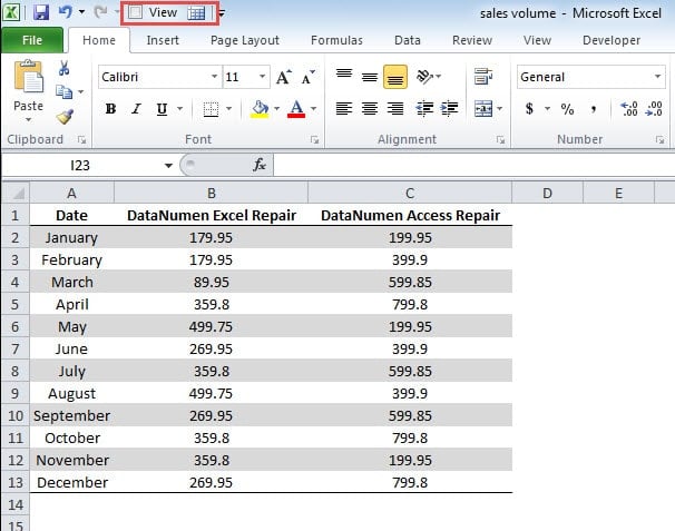
- After that, click the button “OK” in the window. Thus, you have added the buttons in the quick access toolbar.
- Now you can directly click the button in the quick access toolbar to show or hide gridlines.
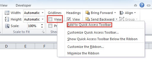
Instead of adding buttons in the “Excel Options” window, you can also add it from the toolbar directly.
- Right click the option “View” or “Gridline” in the first method.
- And then choose the option “Add to Quick Access Toolbar”.
Thus, the button will also appear in the quick access toolbar. You may follow these steps and add buttons quickly.
Method 3: Use VBA Process
Instead of using the above two methods, you can also use the VBA codes to fulfill the task.
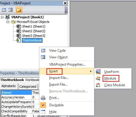
- Press the shortcut “Alt + F11” on the toolbar to open the Visual Basic Editor.
- And then right in the VBA project.
- In the menu, move your cursor on the option “Insert”.
- Next click the option “Module” in the menu.
- Now copy the codes and paste into the new module.
Sub ShowHideGridline()
ActiveWindow.DisplayGridlines = not ActiveWindow.DisplayGridlines
End Sub
- And then press the button “F5” on the keyboard to run the process. You can also click the “Run Sub” in the toolbar. Therefore, you can also use this procedure to show or hide gridlines quickly in your worksheet.
A Comparison of the 3 Methods
You may wonder which method is the most suitable for you. Here we have listed the advantages and disadvantages of the three methods.
| Comparison | Use Features in Toolbar | Add Buttons in the Quick Access Toolbar | Use VBA Process |
| Advantages | This method can be used in other computers. You don’t need to have additional settings. | You can quickly show or hide gridlines by this method. | With just one click,you can show or hide gridlines. |
| Disadvantages | Compared with other methods, there are more steps in this method. | Before you can use the quick access toolbar, you need to spend time to ass buttons into it. | Using VBA codes will make the task more complicated. |
Do Not Lose your Valuable Data Due to an Excel Crash
Excel crash will cause damage to your data and information. Actually, most of the lost data are recoverable as long as you can take the right action. If you don’t know the reason of the corruption, do not try to recovery by yourself. Otherwise, you will lose those precious data forever. At this moment, you can use an Excel repair tool to repair xls data damage. With this tool at hand, you can get back your data and information in a quick time.
Author Introduction:
Anna Ma is a data recovery expert in DataNumen, Inc., which is the world leader in data recovery technologies, including repair doc file problem and outlook repair software products. For more information visit www.datanumen.com
