When an Excel workbook has many worksheets, in order to access them quickly, you may want to create a list of hyperlinks to all worksheets. In this article, we will share 3 methods with you.
If you have an Excel workbook which contains a great amount of worksheets, you may find it troublesome to locate and access your desired worksheet. In this case, you can create a list of hyperlinks to all worksheets, which can let you jump to a specific worksheet simply by clicking on a hyperlink. It’s quite convenient. Thus, here we will introduce 3 ways to create such a list.
Method 1: Manually Create
- For a start, open the specific Excel workbook.
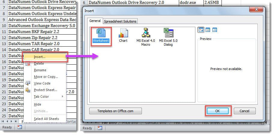
- Then, insert a new sheet before the first worksheet.
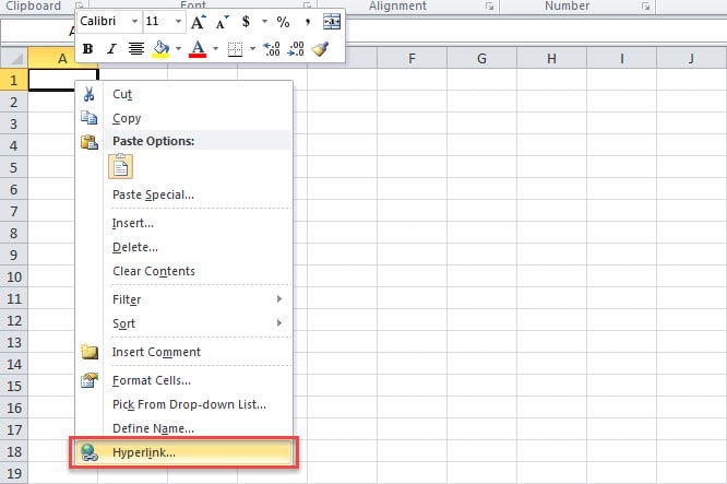
- Next, right click on the Cell A1 and select “Hyperlink” from the context menu.
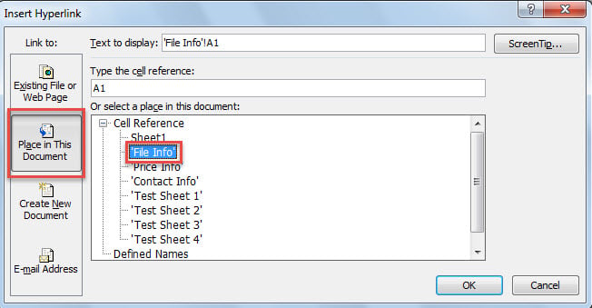
- Later, in “Insert Hyperlink” window, select “Place in This Document” on the left side.
- After that, in the list of “Or select a place in this document”, choose the first sheet except the current new sheet.
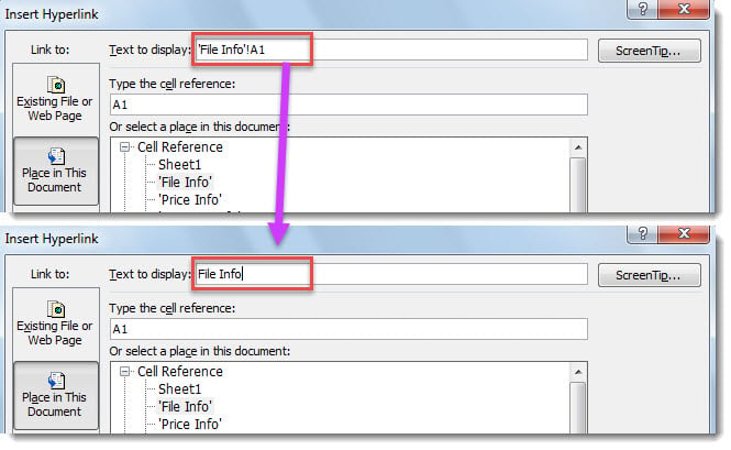
- Then, change “Text to display” to the sheet name.
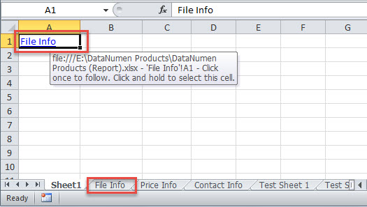
- Finally, click “OK” to insert the hyperlink.
- Now, you can insert the hyperlinks to the remaining sheets one by one.
Method 2: Create via Formula
- First off, create a new sheet.
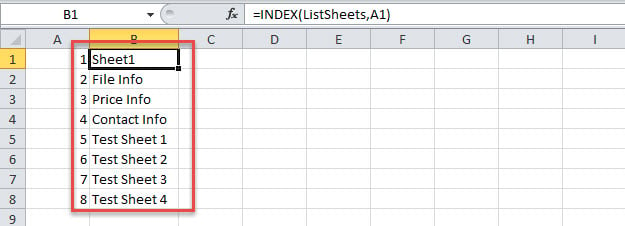
- Then, list all worksheet names according to the Method 2 in the post “3 Quick Ways to Get a List of All Worksheet Names in an Excel Workbook“.
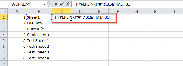
- Later, put the formula below into Cell C1.
=HYPERLINK("#'"&B1&"'!A1",B1)
- Ultimately, drag the function down to get the hyperlinks to the other sheets.
Method 3: Create with VBA
- At the outset, launch Excel VBA editor by referring to “How to Run VBA Code in Your Excel“.
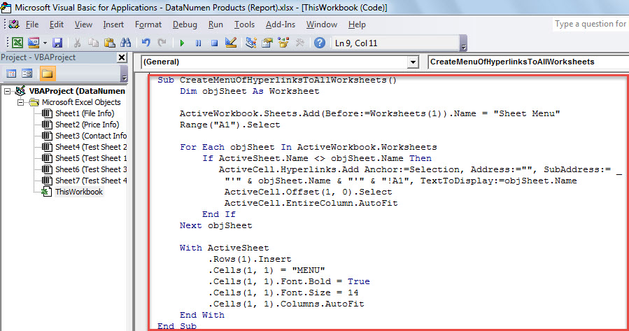
- Then, put the code below into a project or module.
Sub CreateMenuOfHyperlinksToAllWorksheets()
    Dim objSheet As Worksheet

    ActiveWorkbook.Sheets.Add(Before:=Worksheets(1)).Name = "Sheet Menu"
    Range("A1").Select

    For Each objSheet In ActiveWorkbook.Worksheets
        If ActiveSheet.Name <> objSheet.Name Then
           ActiveCell.Hyperlinks.Add Anchor:=Selection, Address:="", SubAddress:= "'" & objSheet.Name & "'" & "!A1", TextToDisplay:=objSheet.Name
           ActiveCell.Offset(1, 0).Select
           ActiveCell.EntireColumn.AutoFit
        End If
    Next objSheet

    With ActiveSheet
         .Rows(1).Insert
         .Cells(1, 1) = "MENU"
         .Cells(1, 1).Font.Bold = True
         .Cells(1, 1).Font.Size = 14
         .Cells(1, 1).Columns.AutoFit
    End With
End Sub
- Next, press “F5” to run this macro.
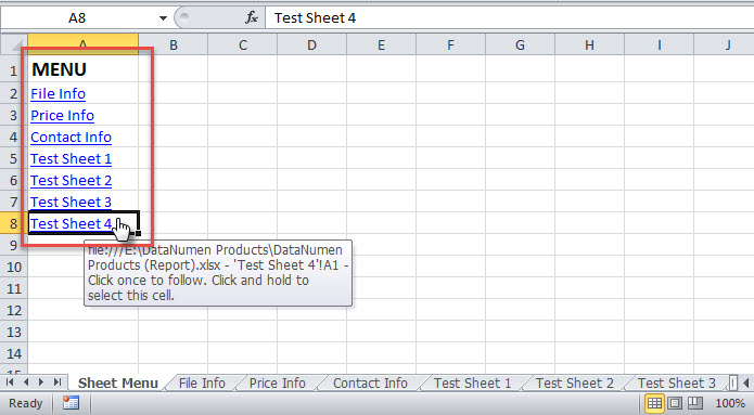
- At once, you will see a new worksheet, which contains all the hyperlinks to all worksheets, like the following screenshot.
Comparison
| Advantages | Disadvantages | |
| Method 1 | Easy to operate | Too tedious if there are too many worksheets |
| Method 2 | Quicker than Method 1 in case of multiple worksheets | Demands you to list numbers and sheet names in advance |
| Method 3 | Much faster and more effective than the above 2 methods | Keep cautious of external macros that may be malicious |
Recover Corrupted Excel Files
Excel can crash from time to time, which can lead to Excel file corruption. Hence, you have to be accustomed to saving the file every time when changing an Excel file. Otherwise, if Excel crashes but you haven’t saved the opened file, you have to resort to xls fix software, such as DataNumen Excel Repair, to get back damaged Excel data.
Author Introduction:
Shirley Zhang is a data recovery expert in DataNumen, Inc., which is the world leader in data recovery technologies, including mdf recovery and outlook repair software products. For more information visit www.datanumen.com
