3 Methods to Sum the Values of the Same Cells in Multiple Worksheets (Part I)

Excel has provided many features for us to calculate data. Here we will introduce 3 useful methods to sum values of same cells in multiple worksheets.

Sometimes in an Excel file, you will need to calculate the total value of certain cells. However, those cells are in several different worksheets. In this image, you can find that there are three worksheets about the sales volume of different sales representative.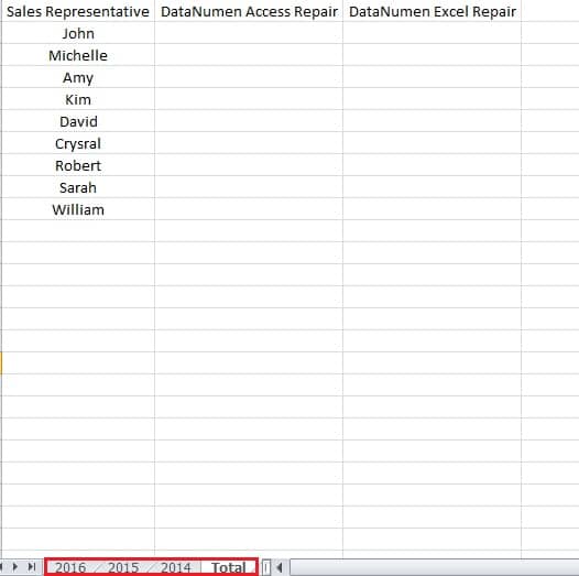

And now you need to sum up the values of each person in the sheet of “Total”. But the original numbers are in the different worksheet. Thus, you can use the following two ways to finish your task.

Method 1: Use SUM Function

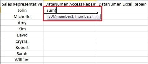
1. In the total worksheet, click the cell B2. And this is the target cell that you want to input the result.
2. Input the following elements into the cell: =sum(
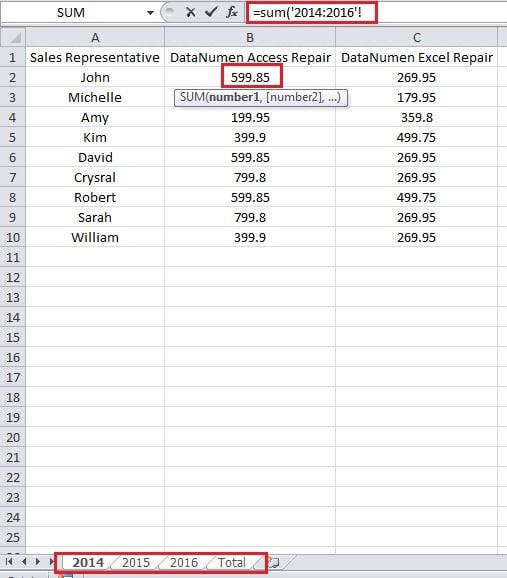
3. Then click the tab of “2014”.
4. Hold the button “Shift” in the ribbon.
5. And then click the tab of “2016”.
6. And then you can release the button of “Shift”.

These 4 steps here mean that you select the three target worksheets. “2014” is the first worksheet and “2016” is the last worksheet. And other sheets between these two will also be selected. You can also see the formula in the Formula Bar.

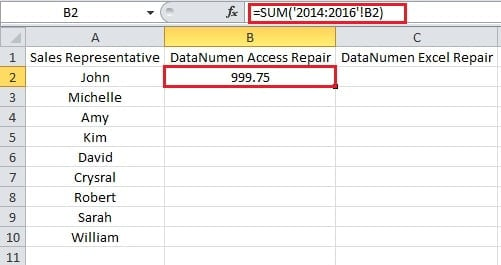
7. Now click the B1 in the interface.
8. Next press the button “Enter”. Thus, you can get the result of the values.
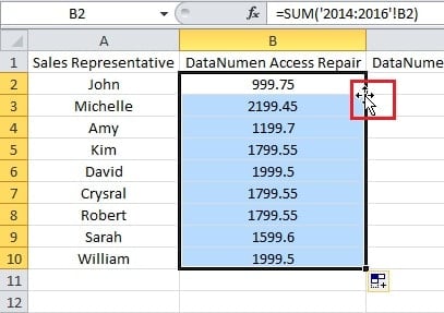
9. Next put your mouse to the bottom right corner.
10. And then double click. Thus, the whole column will be filled with the result.

Method 2: Define Name

This method should also combine the SUM function. And here we will use column C as an example.

1. Click the tab “Formulas” in the ribbon.
2. And then click the button “Define Name”.
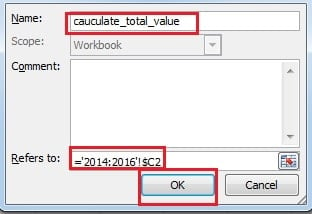
3. In the “New Name” window, input the name into the text box. For example, here we input “cauculate_total_value” into it.
4. As for the “Refers to” text box, first input the “=” into it.
5. Then repeat the step3-6 in the previous part.
6. Next click cell C2. Here you need to delete the second “$” before the number “2”. Because if here you use the absolute reference, you will not be able to insert into the whole column. And of course you can also input into the text box manually.
7. And then click “OK”.
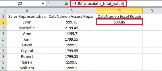
8. Now input the formula into C2.

=SUM(cauculate_total_value)

Thus, you can get the result.

9. Now double click the bottom right corner to insert values into other cells.

What’s more, the above two methods are also called 3-D reference. And it means that the target cell will refer to other cells with the same position in other worksheets.

Except for the 2 methods above, in our next article, we will continue talking about the last method.

Author Introduction:

Anna Ma is a data recovery expert in DataNumen, Inc., which is the world leader in data recovery technologies, including word recovery and outlook repair software products. For more information visit www.datanumen.com