It is easy for you to sort data in a range in the worksheet. Furthermore, now you can also sort data in a column chart by the 2 effective methods that are introduced in this article.
When you demonstrate data and information in a column chart, the order will be the same as in the worksheet. The image below shows such a typical column chart that has the same order with the original range in the worksheet.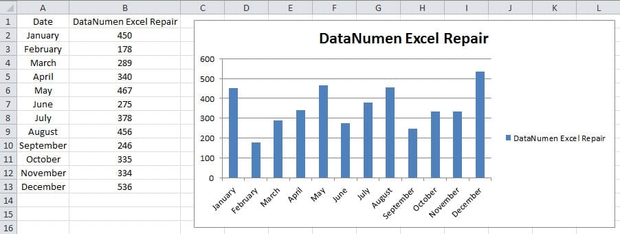
When you need to change the order, or sort the columns in the chart, you may find that you cannot switch the orders of those columns in the column chart manually. But here we have found two effective methods to solve this problem. In the following parts, we will introduce two methods in detail.
Method 1: Sort in the Original Worksheet
When you sort in the original worksheet, the rank in the range will change. But you will also see that the order of columns in the chart will also change accordingly. This is because the data and information in the chart refer to the original area. When this area changes, the chart will certainly change at the same time. Now follow the steps below and see how this method takes effect in a column chart.
- Select the original range in the worksheet.
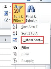
- And then click the button “Sort & Filter” in the toolbar.
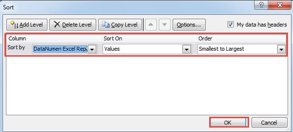
- Next choose the option “Custom Sort” in the drop-down menu. Thus, the “Sort” window will pop up in the worksheet.
- In the “Sort” window, set the criteria that you need. Here we will sort the second column by its values. Besides, the sort order is “Smallest to Largest”. You can also set the criteria according to your actual need and the actual worksheet.
- Next click the button “OK” in the “Sort” window.
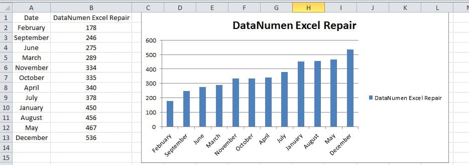
When you click “OK”, you will see the order in the range changes. On the other hand, you will also notice that the order of the columns in the chart also changes at the same time. You may refer to the image below and see the result.
Thus, whenever you need to sort in the chart, you can first sort in the original worksheet.
Method 2: Sort in a Pivot Chart
Except for the above methods, here you can also use this method. By creating a pivot chart in your worksheet, you can sort directly in the chart. And all the chart functions in the pivot chart are the same as the chart functions of an ordinary chart.
- Select the target range in the worksheet.
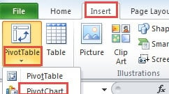
- And then click the tab “Insert” in the ribbon.
- After that, click the small arrow button under the button “PivotTable”.
- Next you will see a drop-down menu with only two options. In this step, you need to select the second option “PivotChart”.
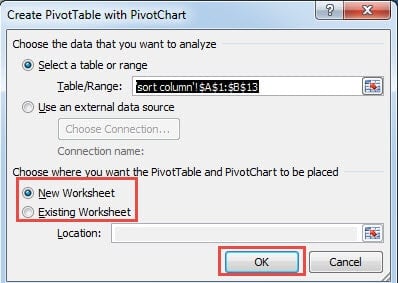
- And then you will see the “Create PivotTable with PivotChart” window pop up in the worksheet. Because we have selected the area in step 1, here you don’t need to select the range again. Of course of you skip step 1, here you can also input the range reference into the text box. Besides, you can also use your mouse to select the range directly.
- Now you need to decide where you want to put the pivot chart. You can either put it in a new worksheet, or you can put in the existing worksheet. Here we choose the first option “New Worksheet”. On the other hand, if you need to put into an existing worksheet, you need also input the location into the corresponding text box. And you can use your mouse to choose the exact location.
- When you finish the setting of the pivot chart, you can click the button “OK” in the window. Thus, you have created a new pivot chart in your current Excel file.
- In the “PivotTable Field List”, choose the field that you need to show in the chart. In this example, we will show the two fields in the chart, thus we check the two options.
- Now click the pivot chart in the worksheet. At the same time, you will see the “PivotChart Tools” tab in the ribbon.
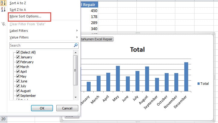
- And then click the field button in the chart on the left bottom area.
- In the new pop-up list, choose the option “More Sort Options”.
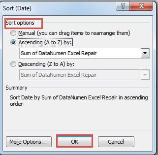
- And then you will see a new window “Sort” pop up. In this window, you can set the options according to your actual need. Here in this example, we will choose the option “Ascending”. And the target column is the “Sum of DataNumen Excel Repair”.
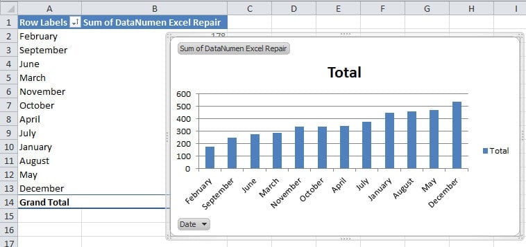
- After that, click the button “OK” on the bottom to finish the setting. Thus, the sort result will appear in the chart. And you will also find that in the original worksheet, the range has already changed accordingly.
This result is the same as sorting directly in the worksheet. Both of the two methods are very useful. And in your actual worksheet, you can choose the most suitable one.
Comparison of the above Two Methods
Now that both of the two methods have the same effect, it’s hard for you to choose which methods that you can use. Here you can refer to the table below. All the advantages and disadvantages we can think of are listed in the table below.
|
Comparison |
Sort in the Original Worksheet |
Sort in a Pivot Chart |
|
Advantages |
1. This method has fewer steps than the second method. Hence, you will find that it is easy to use. And this method is suitable for all the users.
2. You don’t need to add additional chart. The ordinary chart is good enough for you to sort. |
1. In a pivot chart, you can fulfill more other tasks by the unique features. And those features cannot be found in an ordinary worksheet or an ordinary worksheet.
2. All the functions of a chart can also be used in this pivot chart. Therefore, you don’t need to worry about certain manipulations in a chart. |
|
Disadvantages |
1. You cannot directly modify in the common chart itself.
2. Compared with a pivot chart, there is less functions in the ordinary chart. |
1. This method contains more steps than the first method.
2. You need to create an additional pivot chart in the file. And this will add the storage in the file. |
Now you must have a comprehensive understanding of the two different methods. If you want to use easier manipulations, you can use the first methods. If you need to change in the chart and use more features, you can use the second methods. The choice totally depends on your actual need. The method that can help you finish tasks easily and quickly if the best choice for you.
The Reason for Excel Corruption is Detectable
Excel corruption will certainly contains some deep reasons. And almost all the reason for Excel corruption is detectable with today’s technology. The moment you meet with Excel corruption, you need to find the reason. Thus, you can use the right method to repair Excel. When you figure out the reason, it will be much easier for you to find the most suitable solutions.
But if you know nothing about Excel recovery, do not try to repair Excel files by yourself. Incorrect behaviors will cause permanent damage to your precious files. The best choice is turning to professionals for help. In addition, you can use a third-party tool to repair Excel xlsx file corruption. Thus, your data and information will be safe. This tool will be installed on your own computer. Besides, it is easy to operate. Your data and information will not be seen by anyone else because the recovery process is completely going on in your own computer.
Author Introduction:
Anna Ma is a data recovery expert in DataNumen, Inc., which is the world leader in data recovery technologies, including repair Word docx damage and outlook repair software products. For more information visit www.datanumen.com
