Using defined name in Excel can save you a lot of time. Here we will introduce two methods to automatically update the reference range of a defined name in the worksheet.
A defined name has a wide range of use. You can even use a certain name in formulas. The defined named can help you increase your work pace. Sometimes you will certainly add new items into the source range of this name. However, the reference range in the name will not update automatically. In order to solve this problem, we will now use the two methods below.
Method 1: Use OFFSET Function for the Name
Usually when you create a name for a range, you will directly use the cell reference. But here you can also use the OFFSET function for the name.
- Select the target range in the worksheet.
- And then click the tab “Formulas” in the ribbon.
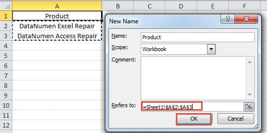
- After that, click the button “Define Name” in the toolbar. Next you will see the “New Name” window pop up.
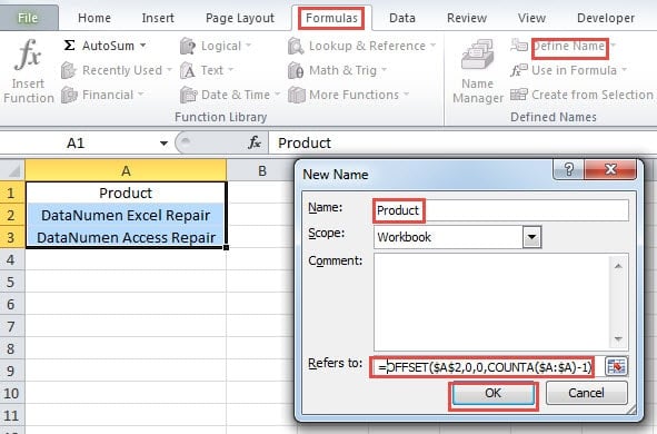
- In this window, the name will automatically appear in the first text box. You can also change it by yourself.
- And then input this formula into the text box of “Refers to”:
=OFFSET($A$2,0,0,COUNTA($A:$A)-1)
You need to modify certain elements according to your need.
- Next click the button “OK” in the window to save this name.
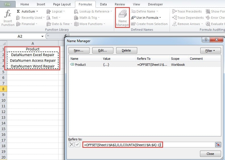
- Now you have finished the setting. You can add new items into the range to have a test. Here we add one new item into cell A4.
- And then click the button “Name Manager” in the toolbar.
- In the “Name Manager” window, click the target name.
- Next click in the “Refers to” text box on the bottom of this window. In column A, there will be dashed box around the new range, which includes the new item that you have added.
Thus, whenever you add new items in the range, this defined name will also update automatically. There is one more thing you need to pay attention. Don’t leave blank cell within the range. And don’t input other items into this column. Otherwise the blank items will also appear in the reference range.
Method 2: Create a Table for the Source Range
Except for the above methods, here you can also use the table for the source range.
- Repeat the first four steps in the previous part and open the “New Name” window.
- And then input the cell reference into the “Refers to” text box. This is the common process of creating a named range.
- In this step, click a cell within the source range. Or you can also select the whole range.
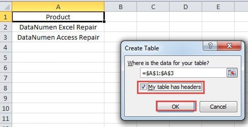
- And then press the shortcut keys “Ctrl +T” on the keyboard.
- In the “Create Table” window, check the option of the headers.
- After that, click the button “OK” to create a table. Now, the settings are OK.
- Here you can also have a test. Inputting a new item into the cell A4. And then you will find that this cell will also be included into the table.
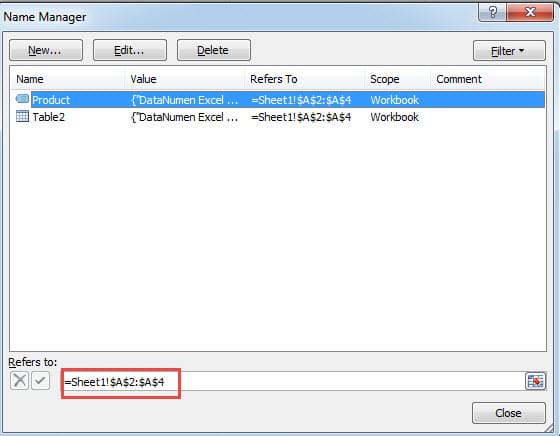
- And then open the name manager.
- Click the target name in this window.
- In the “Refers to” text box, you will find that the range has already updated. This named range also contains the new item.
When using tables, you can input items into other cells in the column. This will not affect the source range.
A Comparison of the two Methods
Here we have listed all the advantages and disadvantages of the two methods.
|
Comparison |
Use OFFSET Function for the Name |
Create a Table for the Source Range |
|
Advantages |
1. Using function can solve the problem when you add or delete items in the source range.
2. Compares with the second method, this method contains fewer steps. |
1. You don’t need to use complex formulas by creating a table.
2. Other cells in the same column will not affect the source range. |
|
Disadvantages |
1. If you don’t know the OFFSET function, you may meet with problems when you need to modify the formula.
2. You also need to make sure that there is no blank cell or additional item in the column. |
1. Creating an additional table will mess up the worksheet, especially when there is a bunch of data and information.
2. There are more steps in this method. You still need to spend a lot of time. |
Data Recovery is not a Cake Walk
When you meet with Excel corruption, you will certainly need to fix it as soon as possible. Most of the time, you will search on the Internet for some advice. However, data recovery is not as easy as you may think. Some incorrect behavior will cause permanent damage to your essential files. You need to consult a data recovery company immediately. And the experienced experts will give you the right suggestion. Besides, in order to repair corrupted Excel quickly, you can also use a powerful third party tool.
Author Introduction:
Anna Ma is a data recovery expert in DataNumen, Inc., which is the world leader in data recovery technologies, including repair Word docx data error and outlook repair software products. For more information visit www.datanumen.com
