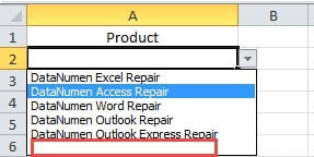
The drop-down list in data validation is a frequently used feature in Excel. In this article, we will introduce two methods to auto refresh the drop-down list.
In our previous article How to Create Drop-down List from a Range of Cells in Your Excel, we have introduced the drop-down list in detail. When the source range changes, the drop-down list will also be affected. Whenever you add or delete an item in the range, you need to check the drop-down list in the target cell. And this can be very irritating. But now, we have found two effective methods for you. By using those methods, the drop-down list will refresh automatically.
Method 1: Use OFFSET Function
In this method, you can use the OFFSET function in the data validation. The image below is the source range in a worksheet. There are 6 product names in this range.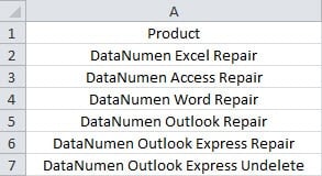
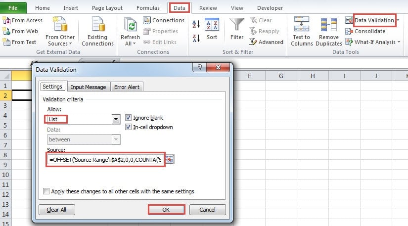
- Click the target cell that you need to create the list. Here we will click a cell A2 in another worksheet.
- And then click the tab “Data” in the ribbon.
- After that, click the button “Data Validation” in the toolbar.
- In the new pop-up window, choose the “List” in the text box of “Allow”.
- And then input this formula into the “Source” text box:
=OFFSET(‘Source Range’!$A$2,0,0,COUNTA(‘Source Range’!$A:$A)-1)
You can change certain elements in the formula according to the actual worksheet.
- And then click the button “OK” in the ribbon to save the setting.
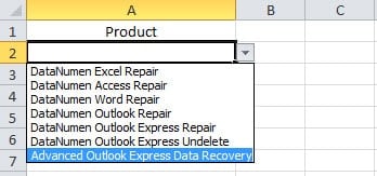
Thus, the drop-down list has been created in the cell. The next time when you add or delete an item in the source range, the items in the list will automatically update. For example, we add a new item into the original range in cell A8. And there are 7 items. In the drop-down list, you can also see 7 items.
The next time you need to create a drop-down list and refer to another range, you can use this method. But by using this method, you need to make sure that there is no additional item in the same column or blank item within the range.
Method 2: Define Name and Use Table
Except for using formula, you can also create a table in the worksheet and define name for this range.
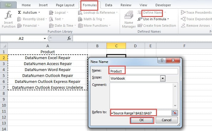
- Select the source range.
- And then click the tab “Formula” in the ribbon.
- After that, click the button “Define Name” in the toolbar.
- Next you will see a new window. Input a name into the “Name” Text Box. Here we will input “Product”.
- And then input the range into the “Refers to” text box.
- Next click the button “OK” to save the range.
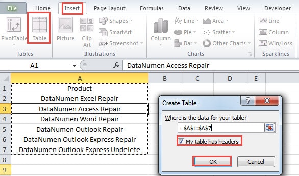
- In this step, click a cell within the source range.
- And then click the tab “Insert” in the ribbon.
- After that, click the button “Table” in the toolbar.
- In the “Create Table” window, check the option of headers according to your need.
- Next click the button “OK” to save the setting.
- Now click the target cell that you need to create the drop-down list.
- Repeat the step 2-4 in the previous part.
- And then input this formula into the “Source” text box:
=Product
This is the define name that you have created in step 4.
- Next click “OK” to save the data validation.
And now you have finished the setting. The next time when you add a new item in the source range, the drop-down list will also update. When you need to delete an item, remember to delete the table row. Otherwise there will be a blank item in the list.
A Comparison of the Two Methods
Both of the two methods are very effective. But still they have advantage sand disadvantages. You can also refer to the table below.
|
Comparison |
Use OFFSET Function |
Define Name and Use Table |
|
Advantages |
1. This method contains fewer steps. And it is easy to perform.
2. By using the function, the worksheet will not be in a mess. |
1. By using this method, you can still input items in other cells in the same row or column.
2. When you also need to use table or define name, you can save a lot of time on those other tasks. |
|
Disadvantages |
1. If you are not familiar with the OFFSET function, you may meet with errors when modify the formula.
2. When there are other items or blank cells in the range, the drop-down list will be in a mess. |
1. There are more steps in this method. You may spend more time on performing the process.
2. When you delete items, you need to delete the table row instead of only the value. |
The next time you need to create the drop-down list which can update automatically, you can choose one of the method. Both of them are very effective.
Fix Excel File Errors
Sometimes you will meet with Excel corruption. And those data disaster can be caused by many different reasons. Before you fix those errors, you need to figure out the reasons. However, if you know nothing about data recovery, do not try to fix the Excel files by yourself. You can consult a sophisticated recovery company for help. Besides, you can also invest an Excel repair tool. This tool is able to repair damaged xls data easily and quickly. Thus, you will get all the data and information back from those corrupt files.
Author Introduction:
Anna Ma is a data recovery expert in DataNumen, Inc., which is the world leader in data recovery technologies, including repair Word docx file error and outlook repair software products. For more information visit www.datanumen.com
