In an Excel worksheet, you may need to extract numbers from values in cells. And in this article, we will introduce you two methods to extract numbers from Excel cells.
There are many cases that both numbers and texts are in same cells. In order to better analyze those values, you will need to extract the numbers and texts. The image below shows such an example. In column A, there are the ID and the name of products.
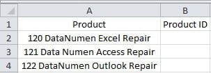
Now you need to input the product ID into column B in the worksheet. And below are the two methods that you can use.
Method 1: Excel Functions
In this part, we will show you how to use Excel functions to extract numbers from cells.
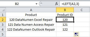
- Click the target cell where you need to input the numbers. In this example, we select cell B2.
- And then input the formula into the cell:
=LEFT(A2,3)
- After that, double click the fill handle of cell B2 and fill the same formula for the whole column. You will see that all the numbers will appear in column B.
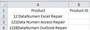
You may find that in this example, all the numbers have the same digits. What if there are other forms of numbers in cells? Actually, there can be countless of number forms in cells. It is impossible to list all of them in just one article. And below we will have another example for you. In this image, the number digits are different for different products.
The function LEFT cannot take effect for all the different cells.
- Input another formula in cell B2:
=MID(A2,1,COUNT(1*MID(A2,ROW($1:$50),1)))
- And then press the shortcut keys “Ctrl +Shift +Enter” on the keyboard. By pressing these shortcut keys combo, this formula will turn into an array formula.
- Next double click the fill handle to fill the formula in the column.
In this formula, the 50 in the “ROW($1:$50)” is an estimated number. You can certainly change into other numbers according to the actual cell. This formula will first count how many numbers in the cell. And then the array formula will connect those numbers. Therefore, even if the number digits are different, you can still use this formula for this column.
When there are other forms of numbers in cells, you can also use functions. But the function may be very complex.
Method 2: VBA Macro
Except for using Excel functions, you can also use VBA to finish this task.
- Press the button “Alt + f11” on the keyboard.
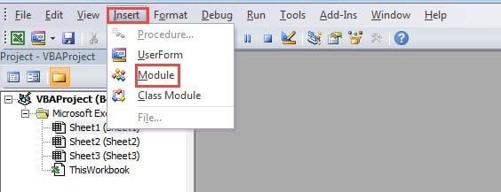
- And then insert a new module.
- Now input the following codes into the new module:
Sub ExtractNumbersFromCells() Dim objRange As Range, nCellLength As Integer, nNumberPosition As Integer, strTargetNumber As String ' Initialization strTargetNumber = "" ' Go through all the cells in the target range For Each objRange In Range("A2:A4") nCellLength = Len(objRange) ' Extract numbers from cells For nNumberPosition = 1 To nCellLength If IsNumeric(Mid(objRange, nNumberPosition, 1)) Then strTargetNumber = strTargetNumber & Mid(objRange, nNumberPosition, 1) End If Next nNumberPosition objRange.Offset(0, 1) = strTargetNumber strTargetNumber = "" Next objRange End Sub
You need to modify the range in the codes according to the actual worksheet.
- After that, run this macro. You can click the button “Run Sub” in the toolbar to run this macro. Besides, you can also press the button “F5” on the keyboard to run it.
- Next come back to the worksheet. You will find that all the product IDs are already in column B.
Even if there are other forms of numbers in cells, the numbers can be extracted by this macro. Therefore, this method is also very convenient.
A Comparison of the Two Methods
In the table below, we have found all the advantages and disadvantages of the two methods.
Comparison |
Excel Functions |
VBA Macro |
Advantages |
1. By using formulas, you can get the numbers in a column that even contains thousands of cells.
2. If you are not familiar with Excel VBA, this method can be your first choice. |
1. You can easily get the result by just one click in the editor.
2. Even if there are other forms of numbers, you can also extract them easily. |
Disadvantages |
1. The results are produced by formulas. You still need to copy and paste them as values.
2. When there are other forms of numbers in cells, you need to spend more time on getting a more complex formula. |
1. If you don’t know how to use VBA macro, you will easily meet with errors when running or modifying the codes.
2. |
The next time when you need to extract numbers from cells, you can use either of the two methods according to your need.
Get Your Data Storage in Order
When there are many Excel files in a storage device, you need to get them in order. Otherwise it is easily for you to meet with data disaster. When such accident happens, you can use an Excel recovery tool to repair corrupted xls data. Thus, your data and information will be safe. And the next time, remember to organize your Excel files.
Author Introduction:
Anna Ma is a data recovery expert in DataNumen, Inc., which is the world leader in data recovery technologies, including repair Word doc document error and outlook repair software products. For more information visit www.datanumen.com
below tow you can extract Numbers from A1 Ctrl+Shift+Enter
=IFERROR(MID($A1,SMALL(IFERROR(ROW(INDIRECT(“1:”&LEN($A1)+1))/(ISTEXT(IFERROR(IF((“.”=MID(” “&$A1,ROW(INDIRECT(“2:”&LEN($A1)+2)),1)),IF(–MID(” “&$A1,ROW(INDIRECT(“1:”&LEN($A1))),1),0),–MID(” “&$A1,ROW(INDIRECT(“2:”&LEN($A1)+2)),1)),””))ISTEXT(IFERROR(IF((“.”=MID($A1,ROW(INDIRECT(“1:”&LEN($A1)+1)),1)),IF(–MID(” “&$A1,ROW(INDIRECT(“1:”&LEN($A1)-1)),1),0),–MID($A1,ROW(INDIRECT(“1:”&LEN($A1)+1)),1)),””))),””),(COLUMN()-COLUMN($B1)+1)*2-1),SMALL(IFERROR(ROW(INDIRECT(“1:”&LEN($A1)+1))/(ISTEXT(IFERROR(IF((“.”=MID(” “&$A1,ROW(INDIRECT(“2:”&LEN($A1)+2)),1)),IF(–MID(” “&$A1,ROW(INDIRECT(“1:”&LEN($A1))),1),0),–MID(” “&$A1,ROW(INDIRECT(“2:”&LEN($A1)+2)),1)),””))ISTEXT(IFERROR(IF((“.”=MID($A1,ROW(INDIRECT(“1:”&LEN($A1)+1)),1)),IF(–MID(” “&$A1,ROW(INDIRECT(“1:”&LEN($A1)-1)),1),0),–MID($A1,ROW(INDIRECT(“1:”&LEN($A1)+1)),1)),””))),””),(COLUMN()-COLUMN($B1)+1)*2-1+1)-SMALL(IFERROR(ROW(INDIRECT(“1:”&LEN($A1)+1))/(ISTEXT(IFERROR(IF((“.”=MID(” “&$A1,ROW(INDIRECT(“2:”&LEN($A1)+2)),1)),IF(–MID(” “&$A1,ROW(INDIRECT(“1:”&LEN($A1))),1),0),–MID(” “&$A1,ROW(INDIRECT(“2:”&LEN($A1)+2)),1)),””))ISTEXT(IFERROR(IF((“.”=MID($A1,ROW(INDIRECT(“1:”&LEN($A1)+1)),1)),IF(–MID(” “&$A1,ROW(INDIRECT(“1:”&LEN($A1)-1)),1),0),–MID($A1,ROW(INDIRECT(“1:”&LEN($A1)+1)),1)),””))),””),(COLUMN()-COLUMN($B1)+1)*2-1)),””)
below two Macros as examples
Public Sub ExtratcNumðwithHelpRow()
Dim TxT() As Variant
Application.ScreenUpdating = False
Application.Calculation = xlCalculationManual
With Worksheets(1)
.Activate
With .Cells(3, 1).Resize(20, 30)
.ClearContents
.Font.Color = vbBlack
End With
With .Range(“B2″) ‘<<<<<<<<<<<<<<<<<<<<<
With .Offset(0, -1).Resize(1, 30)
.ClearContents
.Font.Color = vbBlack
End With
ExtrctNum = "ROW(INDIRECT(""1:""&LEN(" & .Offset(0, -1).Address(False, True) & ")+1))/(ISTEXT(ExtrctNum1)ISTEXT(ExtrctNum2))”
ExtrctNum1 = “IFERROR(IF((“”.””=MID(“” “”&” & .Offset(0, -1).Address(False, True) & “,ROW(INDIRECT(“”2:””&LEN(” & .Offset(0, -1).Address(False, True) & “)+2)),1)),IF(–MID(“” “”&” & .Offset(0, -1).Address(False, True) & “,ROW(INDIRECT(“”1:””&LEN(” & .Offset(0, -1).Address(False, True) & “))),1),0),–MID(“” “”&” & .Offset(0, -1).Address(False, True) & “,ROW(INDIRECT(“”2:””&LEN(” & .Offset(0, -1).Address(False, True) & “)+2)),1)),””””)”
ExtrctNum2 = “IFERROR(IF((“”.””=MID(” & .Offset(0, -1).Address(False, True) & “,ROW(INDIRECT(“”1:””&LEN(” & .Offset(0, -1).Address(False, True) & “)+1)),1)),IF(–MID(“” “”&” & .Offset(0, -1).Address(False, True) & “,ROW(INDIRECT(“”1:””&LEN(” & .Offset(0, -1).Address(False, True) & “)-1)),1),0),–MID(” & .Offset(0, -1).Address(False, True) & “,ROW(INDIRECT(“”1:””&LEN(” & .Offset(0, -1).Address(False, True) & “)+1)),1)),””””)”
””””””””””””””””””””””””””””””””
.Offset(0, -1).Value = “a. Aa. 8.9 .F.M.D. 123.456 0 1 2 3 4 5 A 1 bb 2.2 ccc 33.3″ ‘<<<<<<<<<<<<<<<<<<>>>>>>>>>>>>>>>>>>>>>>>>>>
””””””””””””””””””””””””””””””””
.HorizontalAlignment = xlCenter
.VerticalAlignment = xlCenter
.Font.Color = vbBlue
.FormulaArray = “=IFERROR(MID(” & .Offset(0, -1).Address(False, True) & “,SMALL(IFERROR(ExtrctNum,””””),” & .Offset(-1, 0).Address(True, False) & “*2-1),SMALL(IFERROR(ExtrctNum,””””),” & .Offset(-1, 0).Address(True, False) & “*2-1+1)-SMALL(IFERROR(ExtrctNum,””””),” & .Offset(-1, 0).Address(True, False) & “*2-1)),””””)”
.Replace “ExtrctNum”, ExtrctNum
.Replace “ExtrctNum1”, ExtrctNum1
.Replace “ExtrctNum2”, ExtrctNum2
n = 0
For I = 1 To Len(Range(.Offset(0, -1).Address(False, True)).Value)
t = Mid(Range(.Offset(0, -1).Address(False, True)).Value, I, 1)
If IsNumeric(t) Or (t = “.” And IsNumeric(Mid(Range(.Offset(0, -1).Address(False, True)).Value, I + 1, 1))) Then
TT = TT & t
If (I = Len(Range(.Offset(0, -1).Address(False, True)).Value) And IsNumeric(t)) Then
n = n + 1
ReDim TxT(1 To n) As Variant
TxT(n) = TT
End If
ElseIf TT “” And (IsNumeric(t) = False And IsNumeric(Mid(Range(.Offset(0, -1).Address(False, True)).Value, I + 1, 1))) Then
n = n + 1
ReDim TxT(1 To n) As Variant
TxT(n) = TT
TT = “”
End If
Next
With .Offset(-1, 0)
.Value = 1
.Font.Color = vbBlack
.AutoFill Destination:=.Resize(1, UBound(TxT)), Type:=xlFillSeries
End With
.AutoFill Destination:=.Resize(1, UBound(TxT)), Type:=xlFillCopy
Application.Calculation = xlCalculationAutomatic
Application.ScreenUpdating = True
With .Offset(0, -1).Resize(1, 30)
.EntireColumn.AutoFit
End With
End With
End With
End Sub
Public Sub ExtractNum()
Dim TxT() As Variant
Application.ScreenUpdating = False
Application.Calculation = xlCalculationManual
With Worksheets(1)
.Activate
With .Cells(3, 1).Resize(20, 30)
.ClearContents
.Font.Color = vbBlack
End With
With .Range(“B1″) ‘<<<<<<<<<<<<<<<<<<<<<
With .Offset(0, -1).Resize(1, 30)
.ClearContents
.Font.Color = vbBlack
End With
ExtrctNum = "ROW(INDIRECT(""1:""&LEN(" & .Offset(0, -1).Address(False, True) & ")+1))/(ISTEXT(ExtrctNum1)ISTEXT(ExtrctNum2))”
ExtrctNum1 = “IFERROR(IF((“”.””=MID(“” “”&” & .Offset(0, -1).Address(False, True) & “,ROW(INDIRECT(“”2:””&LEN(” & .Offset(0, -1).Address(False, True) & “)+2)),1)),IF(–MID(“” “”&” & .Offset(0, -1).Address(False, True) & “,ROW(INDIRECT(“”1:””&LEN(” & .Offset(0, -1).Address(False, True) & “))),1),0),–MID(“” “”&” & .Offset(0, -1).Address(False, True) & “,ROW(INDIRECT(“”2:””&LEN(” & .Offset(0, -1).Address(False, True) & “)+2)),1)),””””)”
ExtrctNum2 = “IFERROR(IF((“”.””=MID(” & .Offset(0, -1).Address(False, True) & “,ROW(INDIRECT(“”1:””&LEN(” & .Offset(0, -1).Address(False, True) & “)+1)),1)),IF(–MID(“” “”&” & .Offset(0, -1).Address(False, True) & “,ROW(INDIRECT(“”1:””&LEN(” & .Offset(0, -1).Address(False, True) & “)-1)),1),0),–MID(” & .Offset(0, -1).Address(False, True) & “,ROW(INDIRECT(“”1:””&LEN(” & .Offset(0, -1).Address(False, True) & “)+1)),1)),””””)”
””””””””””””””””””””””””””””””””
.Offset(0, -1).Value = “a. Aa. 8.9 .F.M.D. 123.456 0 1 2 3 4 5 A 1 bb 2.2 ccc 33.3″ ‘<<<<<<<<<<<<<<<<<<>>>>>>>>>>>>>>>>>>>>>>>>>>
””””””””””””””””””””””””””””””””
.HorizontalAlignment = xlCenter
.VerticalAlignment = xlCenter
.Font.Color = vbBlue
.FormulaArray = “=IFERROR(MID(” & .Offset(0, -1).Address(False, True) & “,SMALL(IFERROR(ExtrctNum,””””),(column()-column(” & .Address(False, True) & “)+1)*2-1),SMALL(IFERROR(ExtrctNum,””””),(column()-column(” & .Address(False, True) & “)+1)*2-1+1)-SMALL(IFERROR(ExtrctNum,””””),(column()-column(” & .Address(False, True) & “)+1)*2-1)),””””)”
.Replace “ExtrctNum”, ExtrctNum
.Replace “ExtrctNum1”, ExtrctNum1
.Replace “ExtrctNum2”, ExtrctNum2
n = 0
For I = 1 To Len(Range(.Offset(0, -1).Address(False, True)).Value)
t = Mid(Range(.Offset(0, -1).Address(False, True)).Value, I, 1)
If IsNumeric(t) Or (t = “.” And IsNumeric(Mid(Range(.Offset(0, -1).Address(False, True)).Value, I + 1, 1))) Then
TT = TT & t
If (I = Len(Range(.Offset(0, -1).Address(False, True)).Value) And IsNumeric(t)) Then
n = n + 1
ReDim TxT(1 To n) As Variant
TxT(n) = TT
End If
ElseIf TT “” And (IsNumeric(t) = False And IsNumeric(Mid(Range(.Offset(0, -1).Address(False, True)).Value, I + 1, 1))) Then
n = n + 1
ReDim TxT(1 To n) As Variant
TxT(n) = TT
TT = “”
End If
Next
.AutoFill Destination:=.Resize(1, UBound(TxT)), Type:=xlFillCopy
Application.Calculation = xlCalculationAutomatic
Application.ScreenUpdating = True
With .Offset(0, -1).Resize(1, 30)
.EntireColumn.AutoFit
End With
End With
End With
End Sub